Compare data sets

Conventional Analysis

You can compare two groups of data based on the variables associated with the parametric model using the compareParam function. This function takes parameters such as the two groups of data, the probability model that fits each group of data, and the variable to be compared. You can also customize the graph by specifying additional values. For more details, refer to compareParam. You can obtain the names of the variables as follows:

colnames(Wei(B)$table)

## [1] "shape" "scale" "alpha" "fmax"  "UF"    "MF"    "error"

The compareParam function generates a Q-Q plot of the chosen variable. By setting the parameter new.plot to FALSE, you can stack the graphs. You can obtain the details of the t-student test for the difference of means with a 95% confidence level by setting return=TRUE (the graph will be omitted). The confidence level and alternative hypothesis can be modified using the alternative and conf.level parameters, respectively. For more details, refer to compareParam.

compareParam(B, C, fit=Wei, param="shape")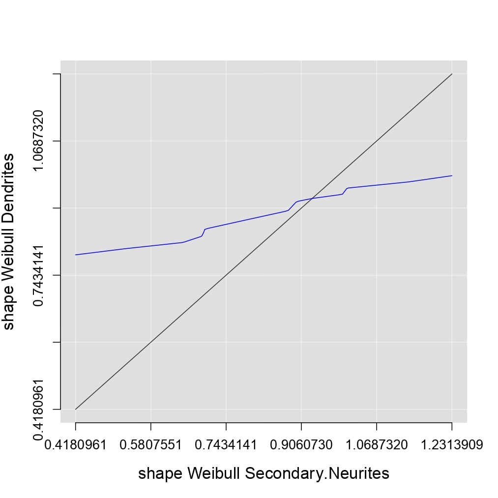

This allows for a conventional analysis of fluorescence recovery, where the immobile fraction (UF) and mobile fraction (MF) are compared. Recall that:

\[UF=\frac{1-f_{max}}{1-f_{min}}\] \[MF=\frac{f_{max}-f_{min}}{1-f_{min}}\] \[UF+MF=1\]

compareParam(B, C, fit=Wei, param="UF", xlim=c(0,1), ylim=c(0,1),lty.lines=c(2,1), col.lines=c("white","red"), lwd.lines=2)
compareParam(B, C, fit=Wei, param="MF", new.plot=F, lwd.lines=2)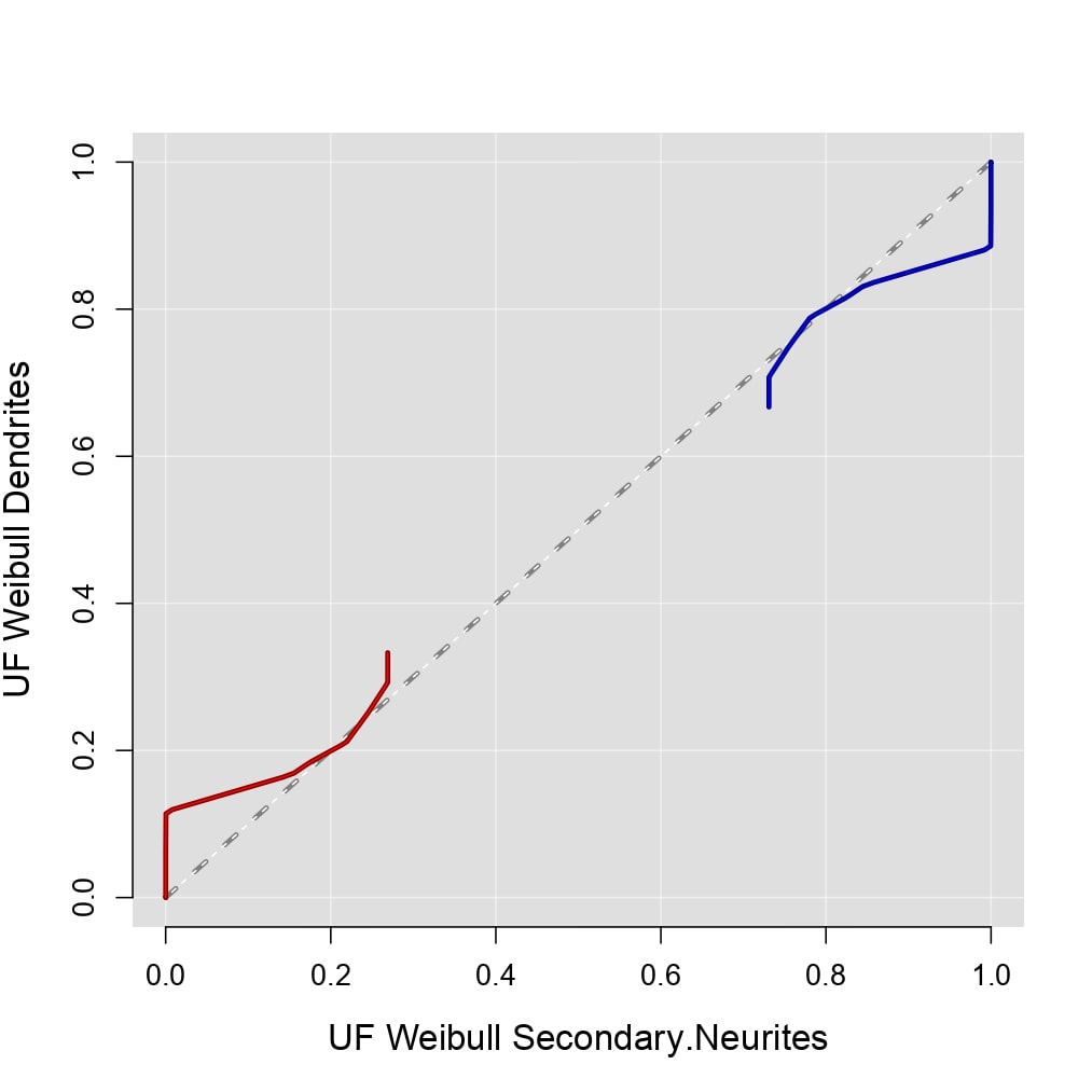

You can also use the compareParam function to compare two probability models fitted to the same group of data based on the error produced by each fit. Note that this graph is already included in the mosaic produced by the compareFit function seen previously.

compareParam(B, B, fit=l(Exp,Wei), param="error", col.lines=c("red", "yellow"), lwd.lines=2, lty.lines=c(2,1), ydigits=2, xdigits=2)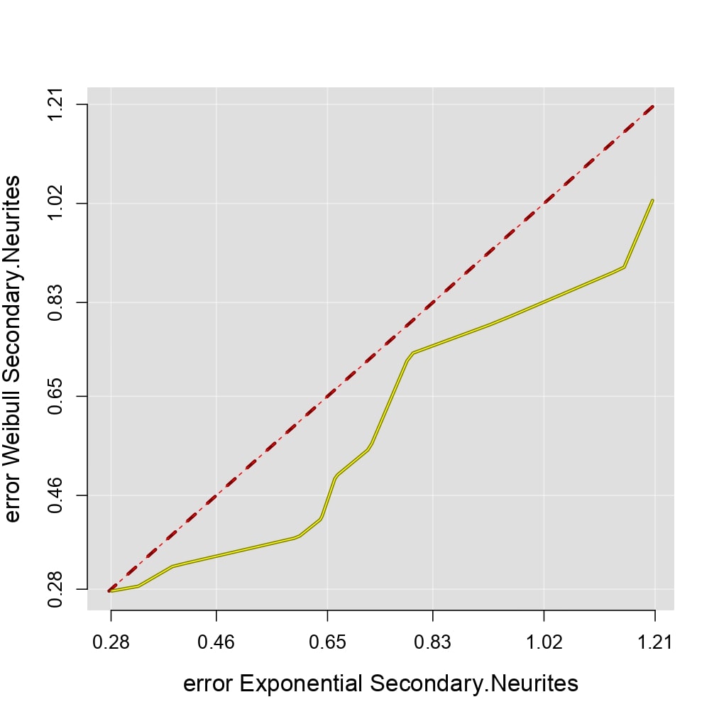

compareParam(B, B, fit=l(Exp,Wei), param="error", return=T)#>>><<<

## 
##  Welch Two Sample t-test
## 
## data:  error_Exponential_Secondary.Neurites and error_Weibull_Secondary.Neurites
## t = 1.2307, df = 21.424, p-value = 0.2318
## alternative hypothesis: true difference in means is not equal to 0
## 95 percent confidence interval:
##  -0.09746458  0.38089484
## sample estimates:
## mean of x mean of y 
## 0.7222331 0.5805180

Mean Behavior Analysis

The analysis of mean behavior involves evaluating the average recovery of fluorescence over time. The mean curve is calculated as follows:

\[\overline F(t)=\frac{1}{n}\sum_{i=1}^{n}F^{AB}_i(t),\]

where \(n\) is the size of the data set, and \(F^{AB}_i\) represents the recovery curve of fluorescence after photobleaching associated with the quantification of fluorescence \(f_i\).

plotFit(B, fit=Wei, plot.lines=T, plot.mean=T, col.mean="purple",lwd.mean=2, xdigits=0, ydigits=2, alp.lines=0.5)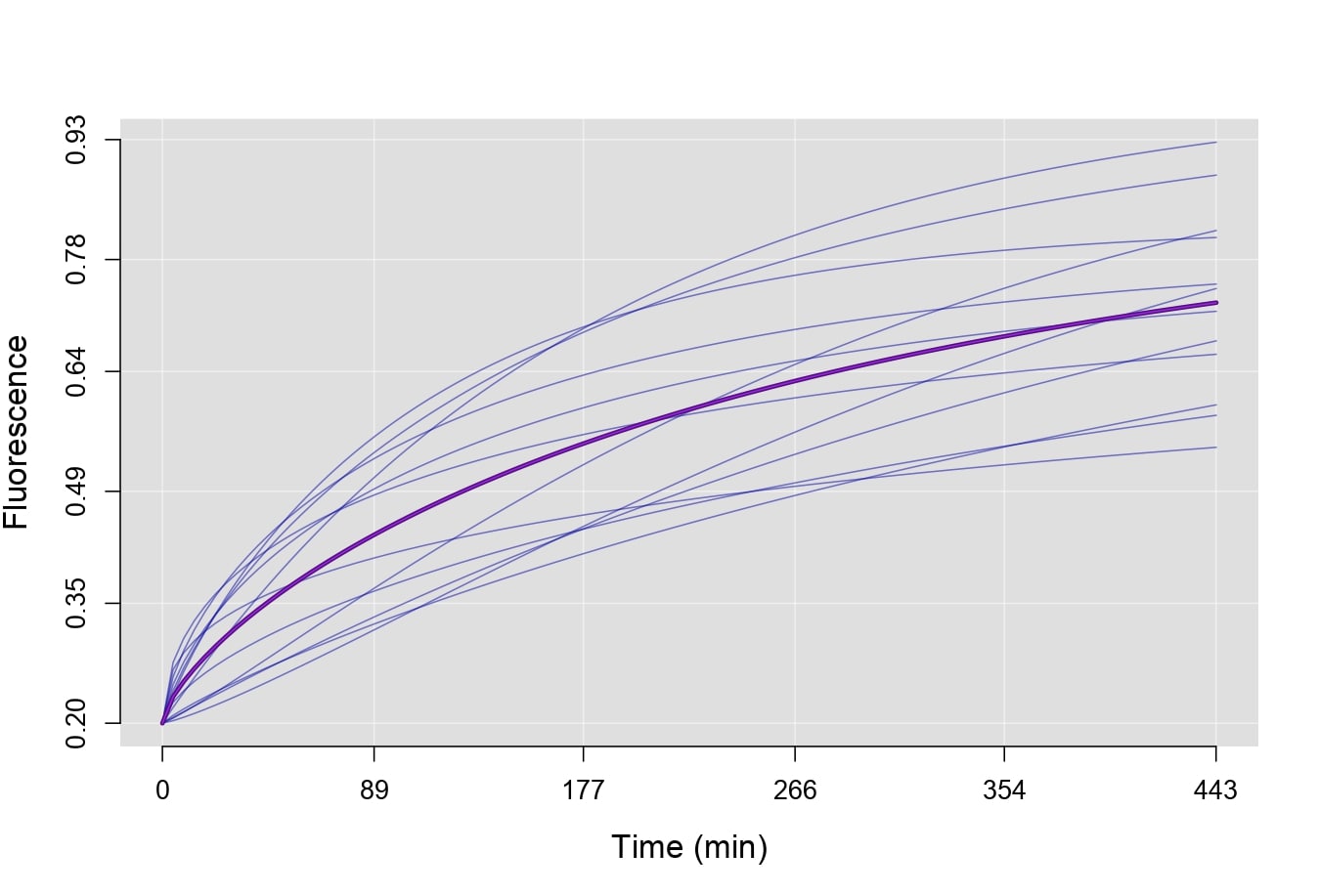

The compareMean function allows you to compare the mean curves of two groups of data using a continuous t-student test for the difference of means over a period of time. The function takes parameters such as the groups of data to be compared, the probability model fitted to the data, and additional values to customize the graph.

The resulting graph represents the p-value of the t-student test, with the reference line indicating the significance level. By setting return=TRUE, you can obtain the details of the test stored in a list (without generating the graph). The confidence level and alternative hypothesis can be modified using the alternative and conf.level parameters, respectively. For more details, refer to compareMean.

compareMean(B, C, fit=Wei, lty.lines=c(2,1), col.lines=c("red","purple"), ydigits=2)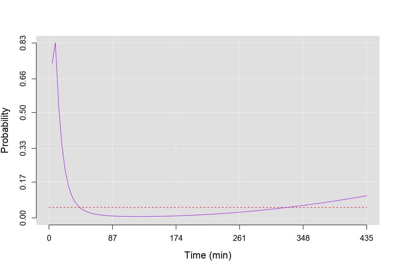

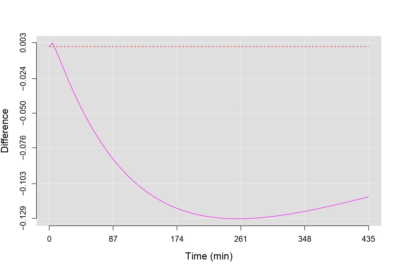
By setting p.value=FALSE, you can calculate the difference of means between the two groups of data, with the reference line located at zero. In this case, by setting return=TRUE, you obtain a vector with the difference of means between the two curves.

compareMean(B, C, fit=Wei, p.value=F, lty.lines=c(2,1), col.lines=c("red","magenta"), ydigits=3)