Appendix

The Fluorescence Recovery Model

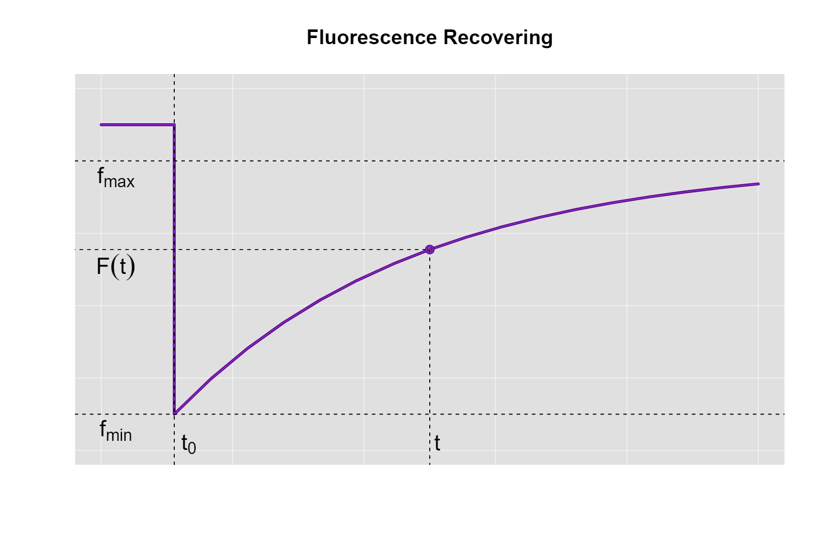
The quantification of fluorescence in the FRAP technique follows a specific recovery pattern. Initially, the fluorescence remains constant, but at the time of photobleaching (also known as \(t_0\)), the fluorescence intensity decreases to a minimum value called \(f_{min}\). From that point on, a gradual process of fluorescence recovery begins, characterized by two fundamental conditions: firstly, the recovery does not decrease as time progresses, and secondly, the fluorescence reaches a maximum limit (\(f_{max}\)) that cannot exceed the initial value before photobleaching. This evolution is graphically represented for a better understanding of the process.

In this sense, the proposed model for fluorescence recovery after photobleaching must comply with the aforementioned characteristics. The general model for fluorescence recovery after photobleaching is as follows:

\[F(t)=f_{min}+\alpha\,(1-f_{min})\,p(t-t_0|\Theta)\]

where \(p\) is a continuous cumulative distribution function (CDF) parametrized by \(\Theta\).

Observations:

• The function \(F(t)\) is defined in the interval \([t_0,\infty)\).

• The value \(f_{max}\) is given by \[f_{max} =\lim_{t\to\infty}F(t)\]

• The value \(\alpha\) is bounded by the values \[\alpha\in[0,1]\]

• The cumulative distribution function \(p\) must be associated with a random variable with support in \((0,\infty)\). Remember that the CDF is defined as follows:

  \[p(t|\Theta)=\int_0^td(x|\Theta)\,\mbox{d}x\] where \(d\) is a parametric density function.

Similarly, the function \(F^{AB}(t)\) is defined to represent the fluorescence recovery curve after photobleaching, which is defined in the time interval \(t\in[0, \infty)\):

\[F^{AB}(t)=f_{min}+\alpha\,(1-f_{min})\,p(t|\Theta).\]

---

Let’s prove that \(F\) satisfies the characteristics of fluorescence recovery after photobleaching:

1. \(F(t_0)=f_{min}\)

   Evaluating:

   \[\begin{aligned} F(t_0) &=f_{min}+\alpha\,(1-f_{min})\,p(t_0-t_0|\Theta)\\ &=f_{min}+\alpha\,(1-f_{min})\,p(0|\Theta)\\ &=f_{min}+\alpha\,(1-f_{min})\int_0^0d(x|\Theta)\,\mbox{d}x\\ &=f_{min}+\alpha\,(1-f_{min})\,(0)\\ &=f_{min} \end{aligned}\] \[\therefore F(t_0)=f_{min}\]

2. \(F(t)\) is non-decreasing

   Consider \(t_1,t_2\in\mathbb R^+\) such that \(t_1\leq t_2\), then

   \[\begin{aligned} t_1-t_0\leq &\;t_2-t_0\\ \Rightarrow p(t_1-t_0|\Theta)\leq &\;p(t_2-t_0|\Theta)\\ f_{min}+\alpha\,(1-f_{min})\,p(t_1-t_0|\Theta)\leq &\;f_{min}+\alpha\,(1-f_{min})\,p(t_2-t_0|\Theta) \end{aligned}\] \[\therefore F(t_1)\leq F(t_2)\]

   The above proves that the parametric model \(F\) is non-decreasing over time.

3. \(f_{max}=f_{min}+\alpha\,(1-f_{min})\) and \(f_{max}\in[f_{min}, 1]\)

   We calculate the limit of \(F(t)\) as \(t\) tends to infinity:

   \[\begin{aligned} f_{max}=\lim_{t\to\infty}F(t) &=\lim_{t\to\infty}f_{min}+\alpha\,(1-f_{min})\,p(t-t_0|\Theta)\\ &=f_{min}+\alpha\,(1-f_{min})\lim_{t\to\infty}\,p(t-t_0|\Theta)\\ &=f_{min}+\alpha\,(1-f_{min})\lim_{t\to\infty}\int_0^{t-t_0}d(x|\Theta)\,\mbox{d}x\\ &=f_{min}+\alpha\,(1-f_{min})\int_0^{\infty}d(x|\Theta)\,\mbox{d}x\\ &= f_{min}+\alpha\,(1-f_{min})\,(1) \end{aligned}\]

   \[\therefore f_{max}=f_{min}+\alpha\,(1-f_{min})\] On the other hand, we have \(\alpha\in[0,1]\), so

   \[\begin{aligned} &0\leq \alpha\leq 1\\ \Rightarrow &0\leq \alpha\,(1-f_{min})\leq 1-f_{min}\\ \Rightarrow &f_{min}\leq f_{min}+\alpha\,(1-f_{min})\leq f_{min}+1-f_{min}\\ \Rightarrow &f_{min}\leq f_{min}+\alpha\,(1-f_{min})\leq 1\\ \Rightarrow &f_{min}\leq f_{max}\leq 1\\ \end{aligned}\] \[\therefore f_{max}\in[f_{min},1]\]

Given a set of fluorescence data \(f\) and a cumulative distribution function \(p(\bullet|\Theta)\), the parameters \((\alpha,\Theta)\) are estimated using the least squares method, which involves minimizing the mean square error between the curves \(f\) and \(F\). The mean square error function is as follows:

\[\begin{aligned}E(\alpha,\Theta)&=\sum_{j=1}^m\left[f(t_j)-F(t_j)\right]^2\\&=\sum_{j=1}^m\left[f(t_j)-f_{min}-\alpha\,(1-f_{min})\,p(t_j-t_0|\Theta)\right]^2\end{aligned}\] where \(\{t_1,t_2,\cdots,t_m\}\) are all the times greater than \(t_0\) quantified for \(f\).

Choosing a Probability Model

The cumulative distribution function \(p(t|\Theta)\) forms the basis for constructing the parametric model of fluorescence recovery \(F(t|\Theta)\). The choice of the function \(p\) is at the discretion of the user, but it is essential that \(p\) has support in \((0,\infty)\). Another aspect that the user must take care of is assigning the intervals where the parameters \(\Theta\) take values. This can be done using the newFit function.

---

Example:

Suppose the user has decided to use a Pareto probability function, then \[p(t|\,\mbox{shape},\mbox{scale})=1-\left(\frac{\mbox{scale}}{t+\mbox{scale}}\right)^{\mbox{shape}}\] \[t>0,\;\;\mbox{scale}>0\;\;\&\;\;\mbox{shape}>0\] We implement the Pareto cumulative distribution function and declare its associated parametric fit:

ppareto <- function(t, shape, scale){
  ppar <- NULL
  for (t in t) 
    ppar <- c(ppar, 1-(scale/(t+scale))^shape)
  ppar
}

Par <- newFit("Pareto", ppareto, c("shape","scale"), list(c(0,a), c(0,b)))

The above code sets \(\mbox{shape}\in(0,a)\) and \(\mbox{scale}\in(0,b)\). After fitting the model Par to a data set, the user needs to verify that the shape and scale values are fully contained within the intervals \((0,a)\) and \((0,b)\), respectively. Otherwise, the user will have to modify the values of \(a\) and/or \(b\) and repeat the process. This can be achieved by visually inspecting the variables returned by the fit: the codes Par(B)$table$shape and Par(B)$table$scale should be executed and the results inspected, where B is a FRAP data set obtained using the newDataFrap function.

---

The functions created by newFit aim to find the best values of \(\Theta\) that minimize the mean square error between the model \(F(t|\Theta)\) and the actual fluorescence recovery data. Therefore, the main criterion for choosing the most suitable probability model \(p\) should be to prefer the model that produces the lowest mean square error. This can be achieved, as seen earlier, using the compareFit function.

compareFit(B, fit=l(Exp, Gam, Wei, Par), col.lines=c("red","yellow"), lty.lines=c(2,1), lwd.lines=2, lwd.mean=2)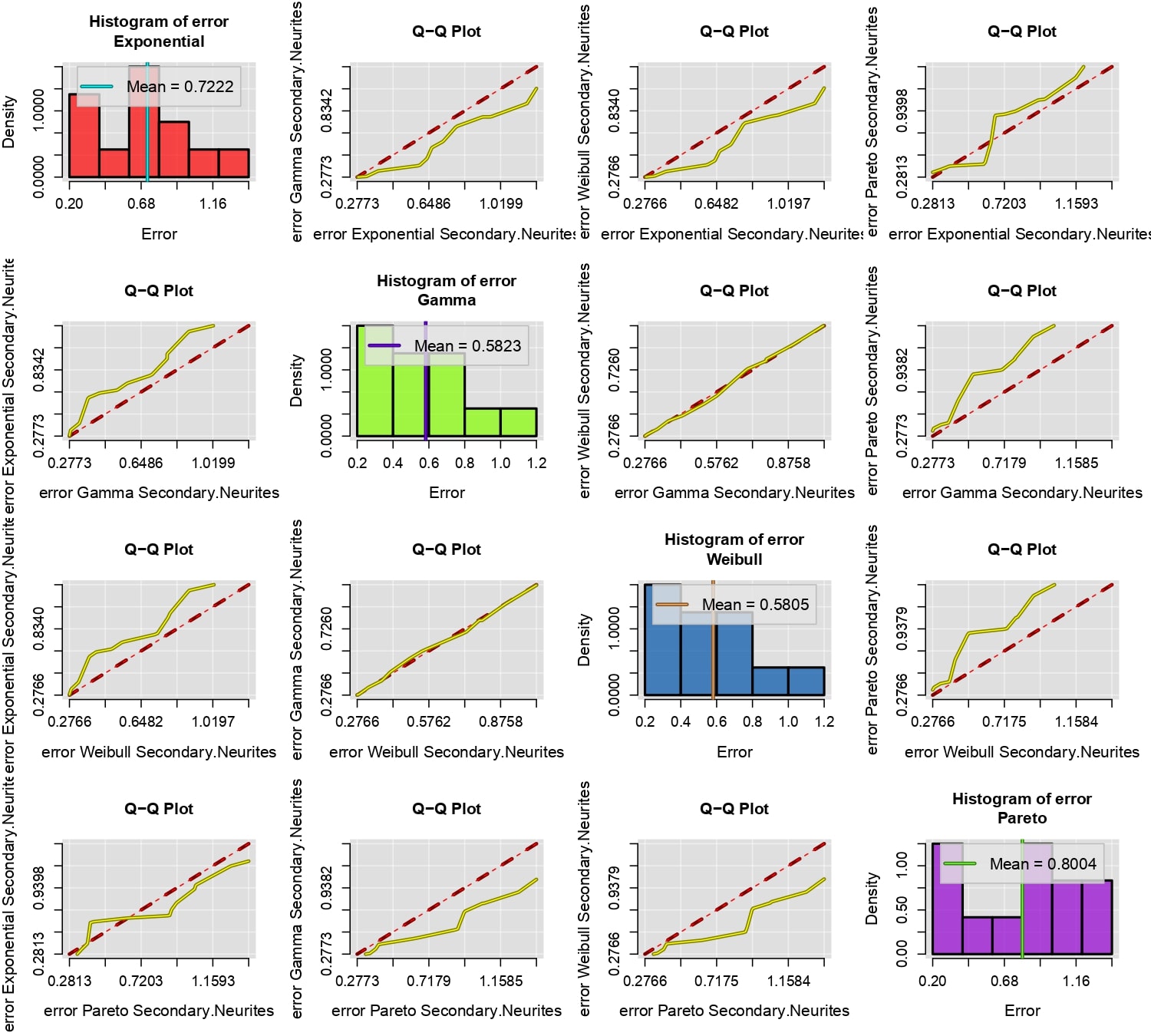

On the other hand, a second criterion for evaluating the viability of a probability model \(p\) is to examine how the simulations of \(F\) behave. If there are discrepancies between the actual fluorescence data and the simulations of \(F\), then it is reasonable to discard the \(p\) model. This would imply that there is no causal relationship between the parameters \(\Theta\) and the fluorescence recovery data. As will be seen in the next appendix, simulations of \(f_{max}\) are particularly sensitive to variations in \(\Theta\).

plotFit(B, B, fit=l(NULL,Exp), col=c("#916F91","#FF4D66"), plot.lines=c(F,T), plot.mean=c(T,F), lwd.mean=2, plot.shadow=c(T,F), lwd.border=1, alp.border=0.4, alp.shadow=0.3, ylim=c(0.2, 1), xdigits=0, simulated=T, seed=1992, main="Exponential simulation", cex.main=1.5)

plotFit(B, B, fit=l(NULL,Gam), col=c("#916F91","#4DB34D"), plot.lines=c(F,T), plot.mean=c(T,F), lwd.mean=2, plot.shadow=c(T,F), lwd.border=1, alp.border=0.4, alp.shadow=0.3, ylim=c(0.2, 1), xdigits=0, simulated=T, seed=1992, main="Gamma simulation", cex.main=1.5)

plotFit(B, B, fit=l(NULL,Wei), col=c("#916F91","#664DFF"), plot.lines=c(F,T), plot.mean=c(T,F), lwd.mean=2, plot.shadow=c(T,F), lwd.border=1, alp.border=0.4, alp.shadow=0.3, ylim=c(0.2, 1), xdigits=0, simulated=T, seed=1992, main="Weibull simulation", cex.main=1.5)

plotFit(B, B, fit=l(NULL,Par), col=c("#916F91","#B34DB3"), plot.lines=c(F,T), plot.mean=c(T,F), lwd.mean=2, plot.shadow=c(T,F), lwd.border=1, alp.border=0.4, alp.shadow=0.3, ylim=c(0.2, 1), xdigits=0, simulated=T, seed=1992, main="Pareto simulation", cex.main=1.5)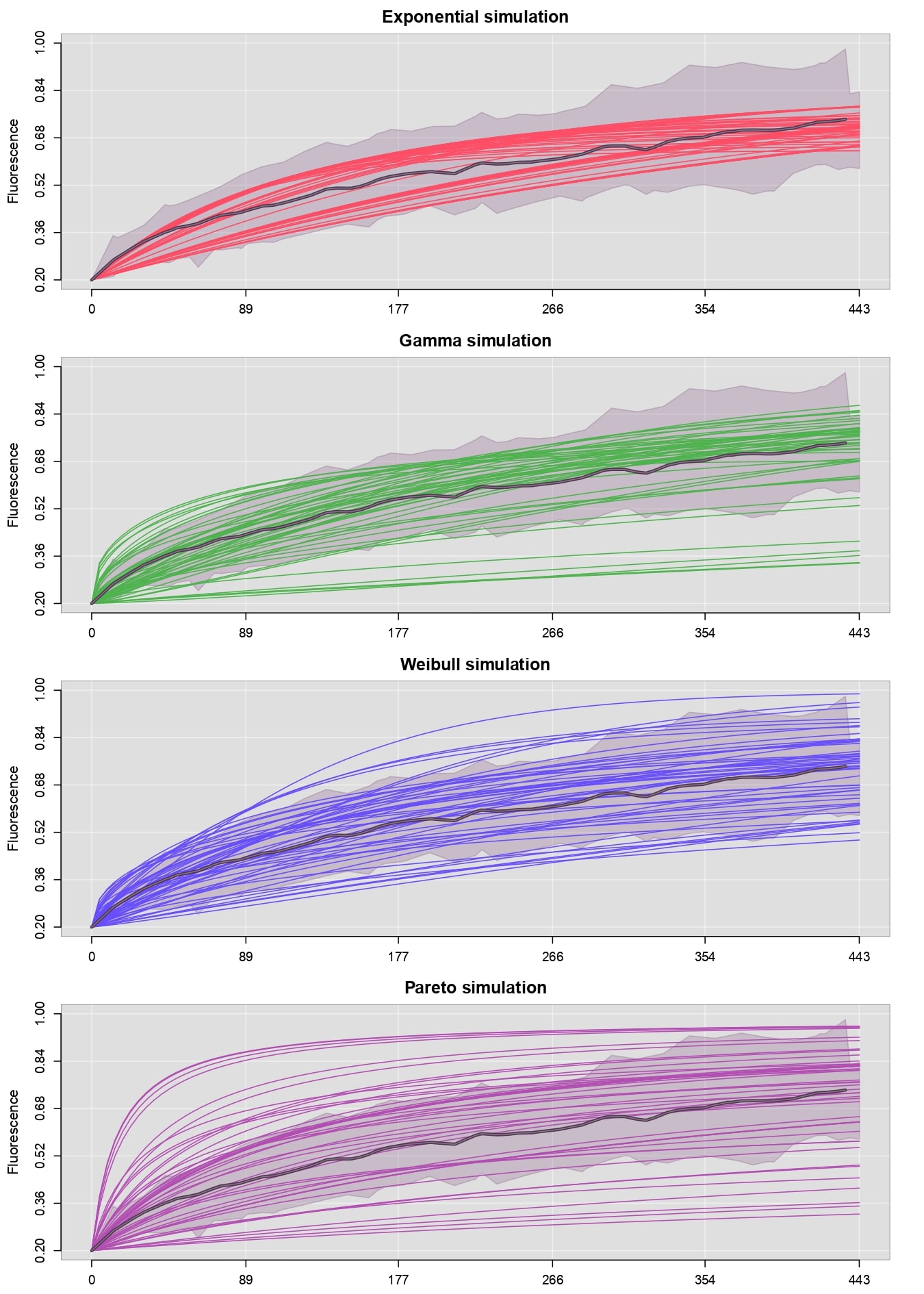

Theory of Stochastic Simulation

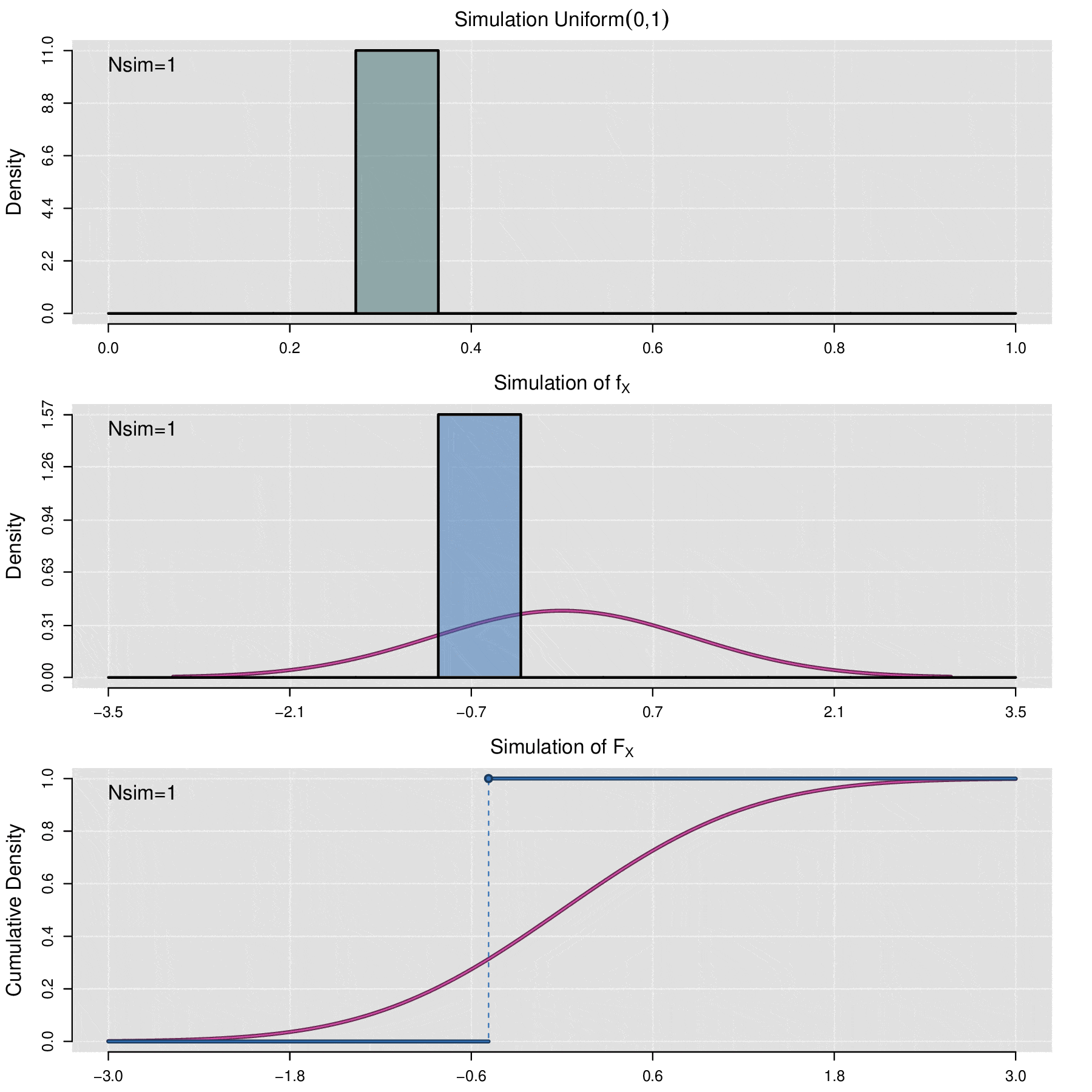
Stochastic simulation is a process by which the behavior of a random variable is reproduced. The basis of simulation follows from the following theorem:

Let \(X\) be a random variable with cumulative distribution function \(\mathbb F_X\), and let \(U\) be a random variable with distribution \(\mbox{Uniform}(0,1)\). Then the random variable \(\mathbb F^{-1}_X(U)\) has the same distribution as \(X\), i.e.,

\[\mathbb F_X = \mathbb F_{\mathbb F^{-1}_X(U)}\]

---

Proof:

\[\begin{aligned}\mathbb F_{\mathbb F^{-1}_X(U)} &=\mathbb P\left[\mathbb F^{-1}_X(U)\leq t\right] =\mathbb P\left[\mathbb F_X\left(\mathbb F^{-1}_X(U)\right)\leq \mathbb F_X\left(t \right)\right]\\ &=\mathbb P\left[U\leq \mathbb F_X\left(t \right)\right] =\int_0^{\mathbb F_X\left(t \right)}f_U(u)\,\mbox{d}u =\int_0^{\mathbb F_X\left(t \right)}1\,\mbox{d}u\\ &=\left.u\right|_0^{\mathbb F_X\left(t \right)}={\mathbb F_X\left(t \right)}-0={\mathbb F_X\left(t \right)} \end{aligned}\] \[\therefore {\mathbb F_X\left(t \right)}=\mathbb F_{\mathbb F^{-1}_X(U)}\]

Note that since \(U\) is a uniform variable, \(f_U(u)=1,\;\; 0<u<1\). (\(f_U\) is the probability density function of \(U\))

---

The above theorem allows us to simulate any random variable \(X\) as long as its cumulative distribution function \(F_X\) is known. Let \(\{u_1,u_2,\cdots,u_n\}\) be a random sample of observed values from the uniform variable \(\mbox{Uniform}(0,1)\). Then \(\{\mathbb F_X^{-1}(u_1),\mathbb F_X^{-1}(u_2),\cdots,\mathbb F_X^{-1}(u_n)\}\) is a sample of simulated values from variable \(X\). In computational terms, to perform the simulation process, generating a random uniform sample is accomplished using pseudorandom number generation algorithms.

There will be situations where it is necessary to simulate the behavior of a data sample \(x_1,x_2,\cdots,x_n\) from an unknown distribution, for which the cumulative distribution function is not available. In these cases, the empirical cumulative distribution function (ecdf) is used for simulation. The ecdf is defined as follows:

\[\widehat{\mathbb F}_{x_1,x_2,\cdots,x_n}(t)=\frac{1}{n}\sum_{i=1}^n\mathbb {I}_{x_i\leq t}\]

where \(\mathbb{I}_{x_i\leq t}=\left\lbrace\begin{aligned} 1,\; x_i\leq t\\ 0,\; x_i> t\end{aligned}\right.\)

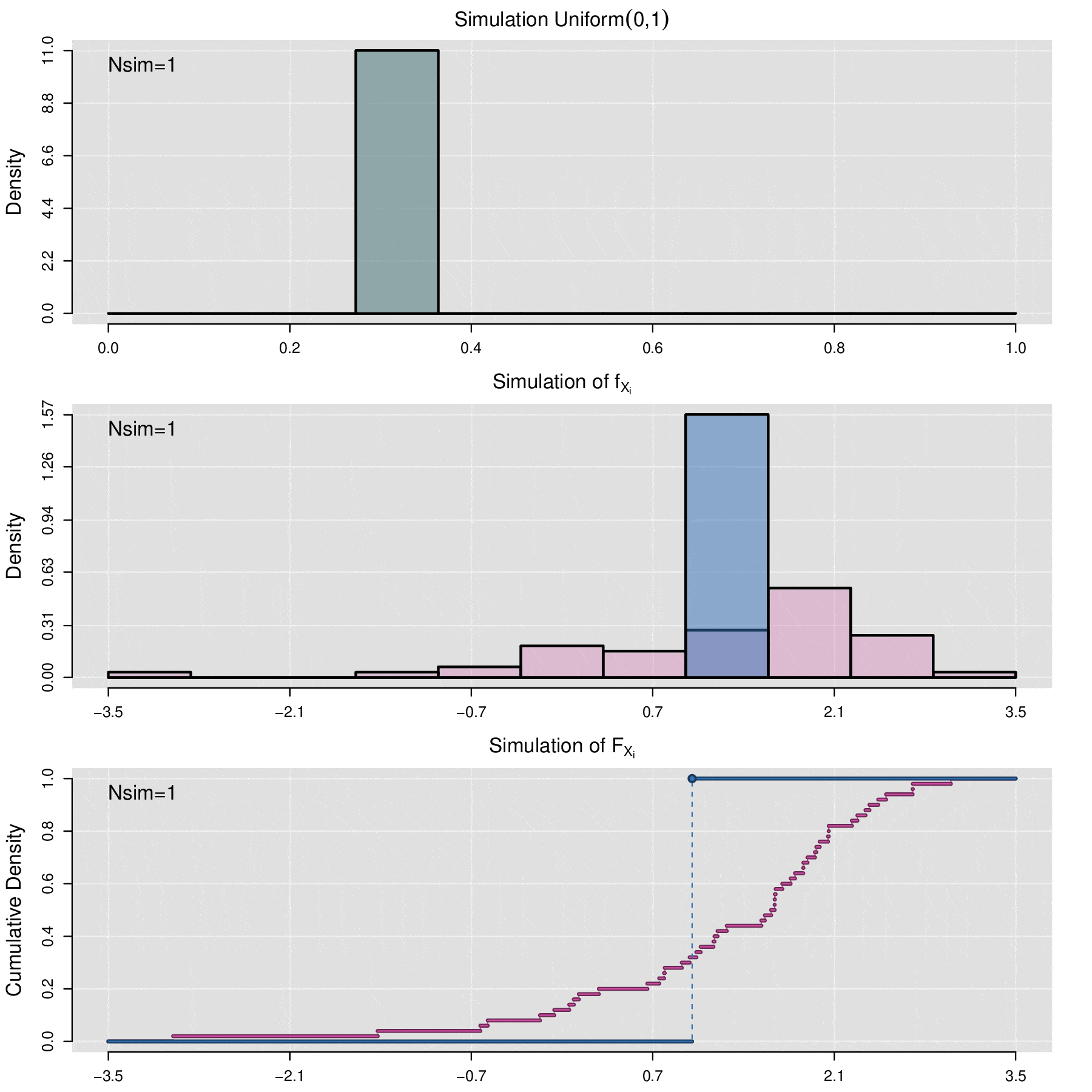
Simulating a FRAP Curve

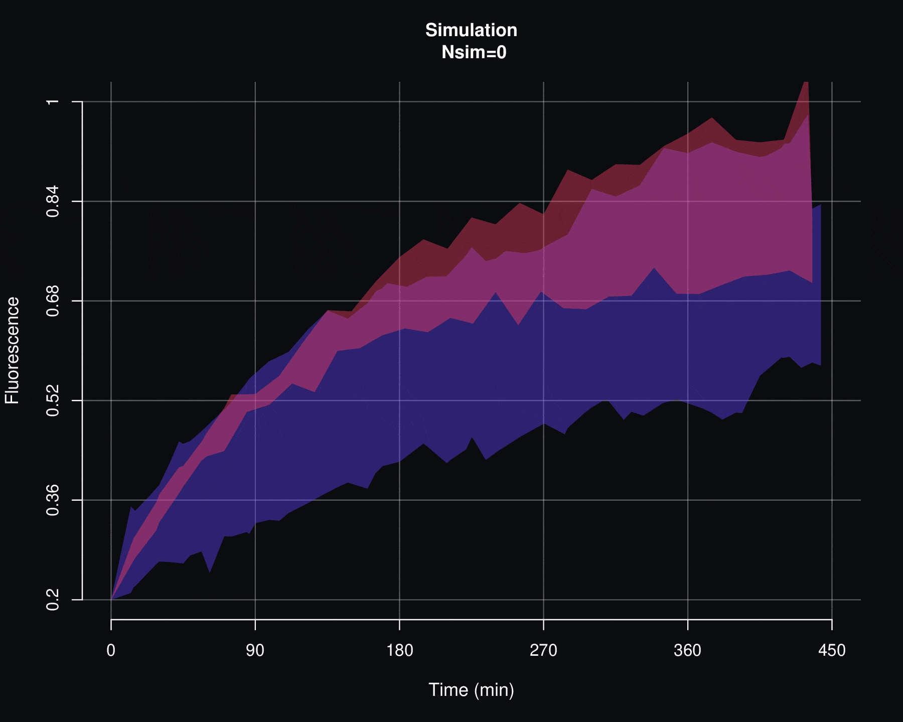
Consider the set of fluorescence quantification data denoted by \(\{f_1,f_2,\ldots,f_n\}\) and the associated FRAP curves \(\{F^{AB}_1,F^{AB}_2,\ldots,F^{AB}_n\}\). The simulation process allows generating a set of \(N_{sim}\) new FRAP curves \(\{\mathcal F^{AB}_1,\mathcal F^{AB}_2,\ldots,\mathcal F^{AB}_{N_{sim}}\}\). Each curve \(\mathcal F^{AB}_j\) is not directly associated with any fluorescence data \(f_i\). Instead, \(\mathcal F^{AB}_j\) is the result of a stochastic simulation process on the set of parameters \(\{(\alpha_1, \Theta_1),(\alpha_2, \Theta_2),\cdots,(\alpha_n, \Theta_n)\}\), where \((\alpha_i, \Theta_i)\) are the values obtained through the least squares optimization between \(f_i\) and \(F_i\).

More specifically, the simulation process for the FRAP curves is as follows:

Using the empirical cumulative distribution function (seen in the previous section of this appendix) of \(\{\Theta_1,\Theta_2,\cdots,\Theta_n\}\), generate the values \(\{ \Theta^{sim}_1,\Theta^{sim}_2,\cdots,\Theta^{sim}_m\}\), i.e.,

\[\Theta_j^{sim}=\widehat{\mathbb F}_{\Theta_1,\Theta_2,\cdots,\Theta_n}^{-1}(U_j)\]

\[\mathcal F^{AB}_j(t)=f_{min}+\alpha_j^{sim}\,(1-f_{min})\,p(t|\Theta_j^{sim}).\]